Introduction of Hierarchical and Partitional Clustering
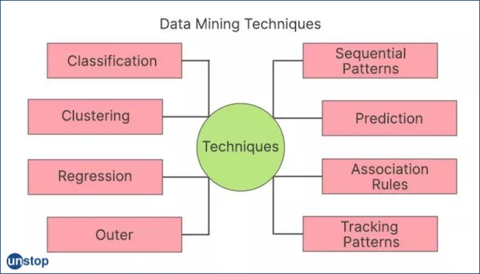
Clustering is a fundamental technique in data analysis that involves grouping similar objects or data points together according to their inherent similarities or dissimilarities. Clustering has proven invaluable in many fields such as machine learning, data mining, pattern recognition, and customer segmentation – just to name a few!
Identifying clusters within datasets, allows analysts to better comprehend underlying structures, uncover hidden patterns, and make data-driven decisions more efficiently.
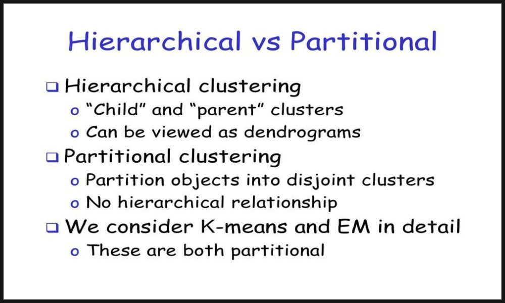
Two common approaches to clustering include hierarchical clustering and partitional clustering. Hierarchical clustering aims at creating a hierarchical structure of clusters, providing a visual depiction of relationships and similarities at different levels of granularity; on the other hand, partitional clustering divides data into an even number of non-overlapping clusters, creating a flat partitioning.
The differences between hierarchical clustering and partitional clustering, from definitions, algorithms commonly employed, processes used, benefits/limitations considered and factors to take into consideration when choosing one over the other. By understanding these distinctions you will gain greater insights into when and how each method can best apply in data analysis tasks.
Definition of hierarchical clustering
Hierarchical Clustering is a data analysis technique used to create hierarchical structures of clusters based on their similarities or dissimilarities, often creating hierarchical pyramids with subclusters at various levels representing various degrees of granularity. Hierarchical Clustering also organizes data points in tree-like structures called dendrograms that serve as visual representations of relationships among clusters and their constituent data points.
Hierarchical clustering can be performed using two primary approaches: agglomerative and divisive. Agglomerative clustering starts by treating each data point as its own cluster and merging similar ones until a termination condition is met, while divisive begins with all points contained within one big cluster and divides it further based on dissimilarity criteria recursively separating into smaller ones; which of these approaches best fits a particular problem and dataset can vary considerably; ultimately it depends on your choice and needs of analysis.
One of the greatest advantages of hierarchical clustering lies in its ability to offer a hierarchical representation of data, enabling exploration at various levels of granularity.This flexibility allows for the identification of both broad and fine-grained clusters within a dataset; additionally, hierarchical clustering does not require pre-specifying the number of clusters as it forms them automatically based on similarities or dissimilarities in the dataset itself.
However, hierarchical clustering does have some drawbacks. It can be computationally expensive when applied to large datasets as its algorithm needs to calculate distances or dissimilarities between all pairs of data points or clusters; dealing with noisy or outlier observations can present further complications as the merging or splitting process could be affected by them; also hierarchical clustering may not work well with mixed data that has complex structures; Hierarchical clustering provides an intuitive, flexible method of grouping data into clusters for insight into its structure and relationships in your dataset.
Definition of Partitional Clustering
Partitional Clustering is a data analysis technique for segmenting datasets into an even number of non-overlapping clusters. This technique seeks to group like data points together while isolating dissimilar ones based on proximity or similarity in multidimensional space. Furthermore, each data point is assigned exactly one cluster, creating an efficient flat partitioning of the dataset.
K-means clustering is one of the most widely-used partitional clustering algorithms. This process starts by randomly initializing K cluster centroids within data space and iteratively assigning each data point to its nearest centroid and updating these centroids based on mean values of assigned data points until convergence occurs, where assignments and centroids no longer differ significantly from one another.
The expectation-Maximization (EM) algorithm is another popular partitional clustering algorithm based on probabilistic modeling using Gaussian mixture models. EM estimates the parameters of Gaussian distributions representing each cluster and assigns data points according to the probability that they belong in that particular cluster; then adjusts both assignment probabilities and cluster parameters until convergence.
Partitional clustering offers several distinct advantages. It is often computationally efficient and scalable when applied to larger datasets due to iterative optimization procedures that utilize iterative data partitioning algorithms. Furthermore, partitional clustering algorithms usually allow for fixed partitioning when desired clusters are known in advance, as well as being flexible enough to handle numerical, categorical, and mixed types of data sets.
However, partitional clustering does have some inherent limitations. It heavily relies on initial positions for cluster centroids or initial parameter estimates that differ across initializations; different initializations can produce drastically different clustering results.
When choosing K, which stands for the number of clusters needed to form optimal clusters. Furthermore, partitional clustering algorithms are particularly sensitive to outliers which could influence centroid calculations or probabilistic assignments that lead to suboptimal cluster formation.
Partitional clustering is a widely utilized technique for subdividing datasets into distinct clusters. It offers efficiency, flexibility, and scalability but requires consideration of initial conditions as well as selecting an optimal number of clusters for data analysis tasks.
Comparison Table of Hierarchical and Partitional Clustering
Sure! Here’s a comparison table highlighting the key differences between hierarchical clustering and partitional clustering:
| Aspect | Hierarchical Clustering | Partitional Clustering |
|---|---|---|
| Cluster Structure | Provides a hierarchical structure of clusters | Provides a flat partitioning of the data into clusters |
| Number of Clusters | No need to pre-specify the number of clusters | Requires pre-specification of the number of clusters (K) |
| Computational Complexity | Computationally expensive for large datasets | Generally more scalable for large datasets |
| Handling Noisy Data | Maybe less robust to noisy or outlier data points | Can be more robust through iterative optimization |
| Flexibility | Enables exploration at different levels of granularity | Provides a fixed partitioning with less granularity |
| Initialization | Initialization is not required | Requires initialization of cluster centroids or parameters |
| Algorithm Examples | Agglomerative clustering, divisive clustering | K-means clustering, Expectation-Maximization (EM) algorithm |
This table summarizes the key distinctions between hierarchical clustering and partitional clustering in terms of cluster structure, the need to specify the number of clusters, computational complexity, handling noisy data, flexibility, initialization requirements, and example algorithms used in each approach.
It provides a concise overview to help you understand the primary differences between these two clustering techniques.
Calculation of distances between data points or clusters
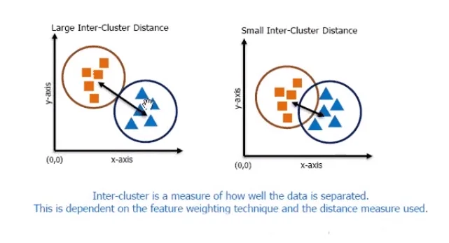
Calculating distances between data points or clusters is a key element of both hierarchical and partitional clustering, enabling an assessment of similarity or dissimilarity between objects or clusters, and aiding in group processes. While the specific methods vary between approaches, here’s an exploration of how they compute distances:
Hierarchical Clustering:
With hierarchical clustering, distances between data points or clusters are measured using various distance metrics such as Euclidean distance, Manhattan distance or cosine distance. Distance metrics depend on the data type and problem at hand; distance calculations typically consider attributes or features associated with data points as they calculate distance.
Initial analyses treated each data point as an individual cluster, and computed distances among all pairs of points. As the clustering algorithm proceeds, its distance calculation process involves choosing from one of three linkage criteria (single linkage, complete linkage, and average linkage), which determines how the distances between clusters are defined based on their constituent data points’ distances from each other.
Partitional Clustering:
With partitional clustering, distance metrics such as Euclidean distance or Manhattan distance may also be used to calculate distances between data points or clusters. However, in partitional clustering, the distances are used primarily for assigning data points to clusters and updating centroids or parameters of existing clusters.
Under the K-means algorithm, for instance, distances between data points and cluster centroids are calculated, with points assigned to clusters with closest centroid. Based on mean or median data point count per cluster, centroid updates accordingly. Iterate until convergence occurs.
Expectation-Maximization algorithms similarly use distance calculations based on probability distributions (e.g., Gaussian distributions) representing each cluster and assign data points according to likelihood or posterior probabilities.
Both hierarchical and partitional clustering rely on distance calculations to assess similarities or dissimilarities among data points or clusters, and play an integral part of clustering algorithms and the clustering process.
Merging or splitting based on distance criteria
Merging or splitting clusters based on distance criteria is an integral step of hierarchical clustering, and affects how clusters are combined or divided based on proximity/dissimilarity criteria.
Let’s explore this technique further:
Agglomerative Clustering: With Agglomerative Hierarchical Clustering, which takes a bottom-up approach, clusters are iteratively combined using distance criteria until each data point has been considered as its own cluster.
Distance metrics such as Euclidean distance or other suitable measures based on data type are used to compute the distance between pairs of clusters. When two clusters come closest together, their closest two members will be combined into one new cluster.=Distances between this new cluster and existing clusters are then recalculated using various linkage criteria (e.g. single linkage, complete linkage, and average linkage).
This process continues until all data points have been merged into one single cluster or until an acceptable termination condition (such as meeting desired number or threshold distance requirements) has been reached.
Divisive Hierarchical Clustering:
With divisive hierarchical clustering, which takes a top-down approach, all data points initially belong to one cluster. To start the clustering process off correctly, each step involves recursively splitting clusters based on distance criteria such as dissimilarity.
At each step distances between data points or clusters are calculated, and then split according to dissimilarity or largest distance criteria; at each step, the data point with the highest dissimilarity or largest distance is chosen for splitting further based on criteria such as threshold distance or desired number of resultant clusters until all data points form their own individual cluster or until termination conditions have been fulfilled – no matter the method employed.
Distance criteria, linkage criteria (for agglomerative clustering), and splitting criteria (for divisive clustering) depends upon the specific algorithm and problem being tackled. Varying clustering results may result from using different criteria; accordingly, the selection should correspond with the goals and characteristics of the data being examined.
Hierarchical clustering uses merging or splitting operations based on distance criteria to form hierarchical structures of clusters. Agglomerative and divisive clustering merge close clusters iteratively while divisive splits dissimilar clusters based on dissimilarity criteria. Specific distance and linkage criteria influence clustering outcomes.
Iterative process until a termination condition is met
Hierarchical clustering and partitional clustering rely on iterative processes until a termination condition is fulfilled, which serves to determine when their algorithms stop processing data and produce their final clustering result.
Let’s explore how each approach defines and applies its termination condition:
Hierarchical Clustering: When employing hierarchical clustering, its termination condition typically depends on either meeting a desired number of clusters or distance thresholds. Clustering iteratively continues until one of these conditions is fulfilled:
Desired number of clusters: When the specified number of clusters has been reached, the algorithm ends. This granularity control allows for precise clustering results.
Threshold distance: When cluster distance exceeds a predefined threshold, the algorithm shuts down. This threshold may represent the maximum dissimilarity that’s acceptable when merging or splitting clusters. Hierarchical clustering allows users to set different termination conditions, which produce clusters at various levels of granularity ranging from coarse-grained clusters to numerous fine-grained ones.
Partitional Clustering: For partitional clustering, the termination condition typically depends upon the convergence of the clustering algorithm. Clustering continues iteratively until convergence has been attained – that is until its results no longer change significantly with subsequent iterations; convergence can be measured by tracking changes to either cluster assignments or centroids/parameters.
Convergence can be defined in various ways depending on the algorithm employed, for instance:
Assignment Stability: The algorithm terminates when cluster assignments no longer change significantly between iterations cycles, or only minimally so.
Centroid Stability: The algorithm ends when any movement or shift of cluster centroids becomes negligible, signifying that their positions have stabilized. Aiming at convergence depends heavily on both the dataset and algorithm’s convergence criteria, with iterations times typically being determined by these. Termination conditions play an essential role in both hierarchical and partitional clustering processes, ensuring they reach a stable state and produce a final clustering result that allows evaluation and interpretation.
No need to pre-specify the number of clusters
Hierarchical clustering does not require pre-specifying the number of clusters; hierarchical clustering algorithms create a hierarchy of clusters without needing to specify an exact count upfront. After clustering has taken place, however, its number can be determined either by looking at a dendrogram or using specific criteria for cluster cutting.
Hierarchical clustering begins by treating each data point as its own cluster, merging similar ones based on proximity or dissimilarity until all points belong to a single one and creating a dendrogram to visualize hierarchical relationships among clusters – this enables visual inspection as well as selecting clusters based on height/level thresholds.
Decisions on how many clusters to create can be guided by domain knowledge, data characteristics, or criteria such as elbow method, silhouette analysis, or gap statistic. These methods assess clustering results at various granularity levels and suggest an ideal number of clusters based on both within-cluster similarity and between-cluster dissimilarity. Hierarchical Clustering does not require predetermining a fixed number of clusters; thus allowing for exploration and the discovery of an optimal cluster count based on dendrogram or specific evaluation criteria.
Ability to explore clusters at different levels of granularity
Hierarchical clustering’s greatest strength lies in its capacity to examine clusters at different levels of granularity. This makes possible examination of results at various resolutions or levels of detail.
Here’s how hierarchical clustering makes possible this ability:
Hierarchical Structure: Hierarchical clustering creates a hierarchical structure of clusters in the form of a dendrogram. This diagram represents merging processes between clusters at various levels and displays their relationships with one another visually. By visually inspecting this dendrogram, clusters can be easily identified.
Dendrogram Cutting: To explore clusters at various levels of detail, cutting the dendrogram can help. Cutting it horizontally at various heights partitions the data into different clusters – higher cuts create less general clusters while lower cuts lead to more specific ones; this cutting process allows you to explore clustering results at multiple resolutions.
Interpretation and Analysis: After cutting your dendrogram at a specific level, you can interpret and analyze its resultant clusters. By exploring their characteristics and patterns within each cluster, observing similarities and differences among them, and deriving insights tailored specifically to that level of granularity you will gain a multi-level view of data for an in-depth understanding of its underlying structure.
Flexibility in Decision-Making: Being able to explore clusters at various levels of granularity allows for more effective decision-making. Depending on your problem or context, you can select the level that is most suited for you – for some analyses a more aggregated view may suffice while for others more fine-grained view might be needed.
Hierarchical clustering provides data analysts with an efficient means of exploring and understanding clustering results at different levels of granularity, providing more thorough analyses and supporting more informed decision-making for the problem at hand.
With its hierarchical structure and dendrogram cutting feature, hierarchical clustering enables data analysts to gain greater control in exploring and comprehending them at various granularity levels. It enables more nuanced analyses while supporting decision-making based on specific needs within their problem context.
Computationally expensive for large datasets
One of the primary limitations of hierarchical clustering is its high computational costs when used on large datasets, particularly when applied to more data points than usual. Hierarchical clustering’s computational cost increases rapidly as more points enter its algorithm; making it less effective compared with some other clustering methods.
Here are a few factors contributing to its cost:
Pairwise Distance Calculation: Hierarchical clustering involves computing pairwise distances among all data points initially, and for large datasets with many points this number increases exponentially; becoming computationally intensive and time-consuming leading to longer execution times as a result.
Memory Requirements: As the data point count grows, so too do memory usage requirements to store pairwise distance values. In large datasets that rely on limited computational resources, this memory usage can become an impediment to progress.
Hierarchical Structure Construction: Establishing the hierarchical structure of clusters requires continuously merging or splitting them using distance criteria until desired clustering results have been reached.
When working with larger datasets, however, this iterative process becomes even more cumbersome and time-consuming resulting in increased computational costs and time taken for completion of clustering process.
Dendrogram Visualization: Visualizing dendrograms can present significant challenges for large datasets when used to examine hierarchical clustering results, due to rendering and interpreting complex dendrograms with numerous data points that may become visually overwhelming and time-consuming. For reducing computational expense, several techniques and optimizations may be used, such as approximate distance calculations, sampling techniques, or parallel processing.
Furthermore, hierarchical clustering algorithms such as BIRCH (Balanced Iterative Reducing and Clustering using Hierarchies) utilize memory-efficient data structures that help manage large datasets efficiently.
Hierarchical clustering may be prohibitively computationally expensive when applied to large datasets, yet remains an effective technique when used with smaller to medium-sized datasets where its cost can be manageable. When dealing with larger datasets it’s essential to be mindful of computational limitations and research alternative clustering methods in order to ensure efficient analysis and scalability.
Difficulty in handling noisy or outlier data points
Hierarchical clustering presents one of the biggest obstacles when it comes to data clustering: its difficulty in handling noisy or outlier data points. Noisy data refers to points that do not conform with the patterns or characteristics found within most of the data, such as outliers that do not follow regular patterns or characteristics found elsewhere; such outliers can significantly impede clustering processes, leading to suboptimal or incorrect results; hierarchical clustering often struggles when dealing with such points:
Sensitivity to Distances: Hierarchical clustering algorithms often rely on distance measures to assess similarity or dissimilarity among data points or clusters, but noisy outliers that differ significantly can distort these measures and alter the clustering outcome; even small numbers of noisy outliers may disrupt the hierarchical structure and cause unexpected merges or splits.
Propagation of Errors: Hierarchical clustering is an iterative process where clusters are combined or split based on proximity or dissimilarity. If noisy data points are incorrectly assigned clusters during early iterations stages, their errors could spread throughout future iterations and have an impactful result for your overall clustering solution.
Linkage Criteria Sensitivity: When choosing hierarchical clustering criteria such as single, complete or average linkage criteria can influence its sensitivity to noisy data. Some linkage criteria are more susceptible than others as they prioritize connections between points that are close together while outliers far apart may create inconsistencies within clustering results.
Dendrogram Cutting Ambiguity: When using a dendrogram to determine the number of clusters, noisy or outlier data points can create confusion when deciding where and how to cut the dendrogram. Outliers may appear as separate branches or subtrees in the dendrogram and contribute to uncertainty in selecting an optimal cutting point and number of clusters.
To reduce the effects of noisy or outlier data points in hierarchical clustering, several strategies can be utilized:
Preprocessing: Employing appropriate preprocessing techniques such as outlier detection and removal or data normalization can help mitigate the effect of noisy data on clustering processes.
Robust Linkage Criteria: Use linkage criteria that are less susceptible to outliers, such as Ward’s linkage which reduces variance within clusters and is therefore more resistant to noise.
Agglomerative Outlier Detection: Utilize outlier detection algorithms as part of hierarchical clustering processes in order to isolate and handle noisy data points separately or exclude them from clustering entirely.
Post-Clustering Analysis: Perform post-clustering analysis to detect and assess the effect of outlier data points or noisy input on clustering results. This process might include looking at cohesion/separation metrics or employing outlier detection algorithms on any newly formed clusters. By employing these strategies, the impact of noisy or outlier data points in hierarchical clustering can be reduced for more robust and accurate clustering results.
Lack of flexibility in accommodating different data types
Hierarchical clustering does have some inherent limitations in terms of accommodating different data types, however. Most hierarchical clustering algorithms assume the data being clustered is numerical and can be represented using distance metrics; this may present difficulties when dealing with categorical, textual, or mixed types.
Here’s why hierarchical clustering may lack flexibility in accommodating different data types:
Hierarchical clustering typically uses distance metrics like Euclidean distance, Manhattan distance, or cosine distance to measure similarity or dissimilarity among data points. While such metrics may work with numeric data sets, categorical or textual data types can present unique challenges when trying to establish meaningful distance measurements between each type. Failure to do so could impair hierarchical clustering’s effectiveness for such diverse cases.
Data Transformation: When applied properly, data transformation techniques can help transform categorical or textual data into a numeric format suitable for distance-based clustering algorithms. Their success and selection depend heavily on each situation based on specific considerations such as data types being transformed causing potential bias or loss of information which could hinder clustering results.
Hierarchical Clustering Doesn’t Handle Feature Selection for Different Data Types: While hierarchical clustering inherently handles feature selection for various data types, hierarchical clustering does not always manage this process of selecting relevant attributes that contribute to clustering. While selecting suitable features depends on data type, selecting suitable features for different data types within a hierarchical clustering framework can often prove challenging.
Domain-Specific Knowledge: Accommodating different data types through hierarchical clustering requires domain-specific expertise and knowledge. Domain experts may need to define custom distance metrics, design specialized preprocessing techniques or implement specific approaches tailored specifically to the characteristics of each data type involved.
To counter the limited flexibility in accommodating different data types, alternative clustering approaches could be explored:
Partitional Clustering: Partitional clustering techniques such as k-means or Gaussian mixture models often offer greater adaptability in accommodating various data types. These methods can accommodate numerical as well as categorical data by employing appropriate distance metrics or probability distributions to suit their characteristics.
Hybrid Approaches: Hybrid clustering approaches utilize multiple algorithms or ensemble techniques to manage diverse data types. By integrating various clustering methods or including domain-specific knowledge into these approaches, they offer greater flexibility and robustness when managing various forms of information.
Preprocessing techniques may also be applied to transform or encode different data types into formats suitable for clustering algorithms, such as one-hot encoding for categorical data or text mining techniques for textual to numerical representations.
Hierarchical clustering may have its limitations in accommodating different data types; alternative clustering approaches and custom preprocessing techniques provide more flexibility and effectiveness in handling diverse datasets. Selecting an effective clustering technique depends on specific factors like data types, problem domain, and desired clustering objectives.
Conclusion
Hierarchical clustering and partitional clustering represent two different approaches to data clustering.
Hierarchical Clustering creates a hierarchy of clusters by iteratively merging or splitting them based on distance criteria. There’s no need to pre-specify their number; you can explore clusters at varying levels of granularity without pre-designating the numbers of clusters beforehand. Computationally intensive solutions may struggle when dealing with noisy or outlier data points.